VGGNet
What VGGNet Does
VGGNet classifies large color images with a deliberately regular pipeline: repeat small convolutions, then halve spatial resolution with max pooling. VGG-16 and VGG-19 became especially common as pretrained feature extractors for detection, segmentation, and style transfer.
Very Deep Convolutional Networks for Large-Scale Image Recognition, by Karen Simonyan and Andrew Zisserman, studied how increasing depth from 11 to 19 weight layers affected ImageNet performance. The models placed first in ILSVRC 2014 localization and second in classification.
Core Idea
Rather than use a single large spatial kernel, stack 3 × 3 convolutions. Two such layers see a 5 × 5 receptive field; three see a 7 × 7 field. The stack uses fewer weights than one 7 × 7 convolution at equal channel width and inserts a ReLU after each layer, allowing richer transformations.
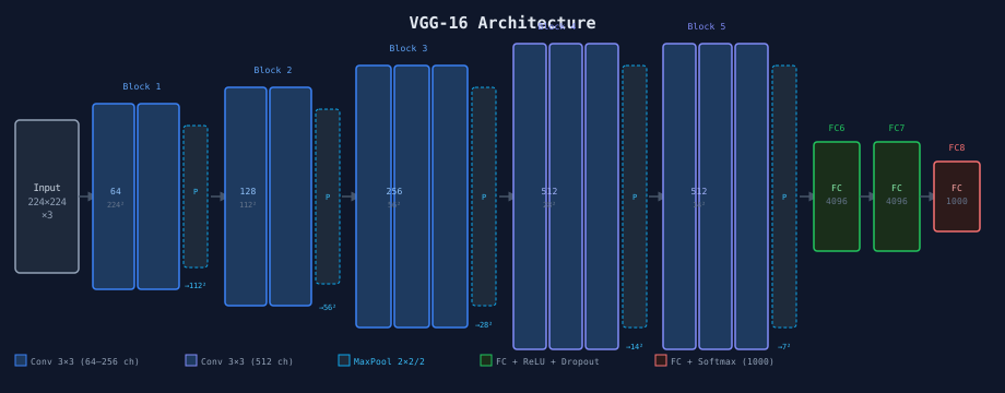
The family includes four main variants, differing only in the number of conv layers per block:
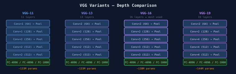
VGG Variants — VGG-11, VGG-13, VGG-16, VGG-19
Source: Simonyan & Zisserman, 2014 — Very Deep Convolutional Networks (ICLR)
How It Works
1. Repeat one simple block pattern
For VGG-16, a 224 × 224 RGB image passes through five convolutional blocks:
| Block | Convolutions | Output after 2 × 2 max pool |
|---|---|---|
| 1 | 2 × Conv3-64 | 112 × 112 × 64 |
| 2 | 2 × Conv3-128 | 56 × 56 × 128 |
| 3 | 3 × Conv3-256 | 28 × 28 × 256 |
| 4 | 3 × Conv3-512 | 14 × 14 × 512 |
| 5 | 3 × Conv3-512 | 7 × 7 × 512 |
Each 3 × 3 convolution uses stride 1 and padding 1, so it preserves width and height. Each pool uses stride 2, halving both. VGG-16 and VGG-19 use 3 × 3 spatial convolutions throughout; the broader experimental family also included a configuration with some 1 × 1 convolutions.
2. Classify the final feature maps
The 7 × 7 × 512 result is flattened and fed to two 4,096-unit fully connected layers with ReLU and dropout, followed by a 1,000-way classifier. These fully connected layers account for most of VGG-16's roughly 138 million parameters.
3. Compare depth systematically
| Model | Weight layers | Convolutions per block | Approx. parameters |
|---|---|---|---|
| VGG-11 | 11 | 1–1–2–2–2 | 133M |
| VGG-13 | 13 | 2–2–2–2–2 | 133M |
| VGG-16 | 16 | 2–2–3–3–3 | 138M |
| VGG-19 | 19 | 2–2–4–4–4 | 144M |
The original experiments found that greater depth generally improved classification within this tested range. That is evidence for depth's value under the study's setup, not a rule that adding layers always improves any network.
4. Train the network
The paper used SGD with momentum 0.9, weight decay , batch size 256, and an initial learning rate of 0.01 reduced during training. Random 224 × 224 crops, horizontal flips, and color variation augment the data. Unlike AlexNet, VGG omitted local response normalization after finding that it did not improve performance.
Why It Works
- Small kernels, larger effective field: A stack captures broad context without paying the parameter cost of one large same-width kernel.
- More nonlinear stages: ReLU between convolutions lets each block represent more complex functions.
- Predictable hierarchy: Pooling trades spatial resolution for more channels and increasingly semantic features.
- Uniform design: Repeated blocks are easy to inspect, implement, and reuse.
- Transferable features: The learned intermediate activations proved useful well beyond ImageNet classification.
Limitations
- VGG-16 has about 138 million parameters, mostly in its classifier, so weights require substantial memory.
- Dense 3 × 3 stacks demand much more computation than later bottleneck or separable-convolution designs.
- The original architecture has no batch normalization; later VGG-BN variants add it.
- No residual path exists, so going far beyond the tested depths introduces optimization and degradation problems.
- The original fully connected head assumes a fixed final feature-map size unless it is converted or replaced.
- Its accuracy has been surpassed, though its simple blocks remain valuable for teaching and feature-based applications.
Related
- LeNet-5
- AlexNet
- ResNet
- CNN
- Convolution
- Pooling
- Dropout
- Activation Function
- ResNet (2015) — residual paths for much deeper networks
- DenseNet (2016) — dense feature reuse
- EfficientNet (2019) — compound scaling
- VGG-BN variants — batch-normalized VGG models
Sources
- Very Deep Convolutional Networks for Large-Scale Image Recognition — Original VGGNet paper by Simonyan & Zisserman (ICLR 2015)
- VGGNet — Wikipedia
- ILSVRC 2014 Results
- CS231n: Convolutional Neural Networks for Visual Recognition — Stanford course notes
- PyTorch VGG pretrained models