AlexNet
What AlexNet Does
AlexNet classifies color photographs into 1,000 ImageNet categories. Its decisive ILSVRC 2012 result reduced top-5 error from the runner-up's 26.2% to 15.3%, showing that a large convolutional network trained on GPUs could outperform the dominant handcrafted-feature systems.
It was introduced in ImageNet Classification with Deep Convolutional Neural Networks by Alex Krizhevsky, Ilya Sutskever, and Geoffrey Hinton. It scaled ideas from LeNet-5 to large, varied RGB images and helped accelerate the adoption of deep learning in computer vision.
Core Idea
Use a much larger CNN, enough labeled data, and GPU computation together. ReLU makes optimization faster, augmentation exposes the model to plausible image variations, and dropout regularizes the parameter-heavy classifier.
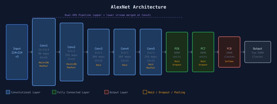
AlexNet Architecture
Source: Krizhevsky et al., 2012 — ImageNet Classification with Deep CNNs (NeurIPS)
Below are representative categories from the ImageNet dataset (ILSVRC 2012) that AlexNet was trained to classify:
How It Works
1. Build a spatial feature hierarchy
AlexNet has five convolutional and three fully connected weight layers. It is commonly described with 224 × 224 crops; reproductions often use 227 × 227 inputs to match the published first-layer dimensions exactly.
| Stage | Main operation | Output in the published layout |
|---|---|---|
| Conv1 | 96 filters, 11 × 11, stride 4; ReLU, LRN, pool | 27 × 27 × 96 after pooling |
| Conv2 | 256 filters, 5 × 5; ReLU, LRN, pool | 13 × 13 × 256 |
| Conv3 | 384 filters, 3 × 3; ReLU | 13 × 13 × 384 |
| Conv4 | 384 filters, 3 × 3; ReLU | 13 × 13 × 384 |
| Conv5 | 256 filters, 3 × 3; ReLU, pool | 6 × 6 × 256 |
| FC6–FC7 | 4,096 units each; ReLU, dropout | 4,096 |
| FC8 | Linear classifier | 1,000 scores |
The large first kernel quickly reduces resolution. Later 3 × 3 layers combine increasingly abstract features. Overlapping 3 × 3 max pooling with stride 2 performs the spatial reductions.
2. Optimize with ReLU and two GPUs
ReLU computes and trained much faster than tanh in the paper's comparison. The original model split feature maps across two 3 GB GTX 580 GPUs, with communication at selected layers, because one device could not hold the complete network.
3. Regularize the large classifier
Random 224 × 224 crops from resized 256-pixel images, horizontal reflection, and PCA-based RGB intensity changes augment the 1.2 million-image training set. Dropout with probability 0.5 is applied to FC6 and FC7. Local response normalization (LRN) follows the first two convolutions, though later architectures generally replaced or omitted it.
4. Train and predict
The roughly 60-million-parameter network was trained with SGD, momentum 0.9, weight decay , batch size 128, and an initial learning rate of 0.01. A softmax converts the final 1,000 scores into class probabilities.
Why It Works
- Scale: ImageNet supplies enough diverse labels to learn reusable visual features.
- GPU training: Parallel convolution makes a model of this size practical.
- ReLU: Its positive-side gradient avoids tanh-style saturation there and speeds training, although it does not eliminate every gradient problem.
- Augmentation and dropout: Both counter overfitting in a network whose fully connected layers contain most parameters.
- Depth: Successive convolutions move from local edges and textures toward object parts and category evidence.
Limitations
- About 60 million parameters and large fully connected layers make the model memory-heavy.
- The architecture's split-GPU groups and other choices reflect 2012 hardware constraints.
- LRN is computational overhead and did not remain a standard component.
- Large early strides discard fine spatial detail.
- Without skip connections, simply stacking many more layers becomes difficult to optimize.
- Newer networks provide better accuracy and efficiency, but AlexNet remains historically and pedagogically important.
Related
- LeNet-5
- CNN
- VGGNet
- ResNet
- Convolution
- Pooling
- Dropout
- Activation Function
- VGGNet (2014) — stacked small convolutions
- GoogLeNet / Inception (2014) — parallel multi-scale branches
- ResNet (2015) — residual connections
- MobileNet — depthwise separable convolutions
Sources
- ImageNet Classification with Deep Convolutional Neural Networks — Original AlexNet paper by Krizhevsky, Sutskever & Hinton (NeurIPS 2012)
- AlexNet — Wikipedia
- ImageNet — Wikipedia
- ILSVRC 2012 Results
- CS231n: Convolutional Neural Networks for Visual Recognition — Stanford course notes