LeNet-5
What LeNet-5 Does
LeNet-5 classifies small grayscale images of handwritten characters. It learns useful stroke patterns directly from pixels, then combines those patterns to choose an output class.
Introduced in 1998 in Gradient-Based Learning Applied to Document Recognition by Yann LeCun, Leon Bottou, Yoshua Bengio, and Patrick Haffner, it was an influential early convolutional network and part of a practical bank-check reading system. Its success helped establish convolution, shared weights, subsampling, and end-to-end gradient-based training as a workable recipe for document recognition.
Core Idea
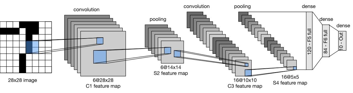
LeNet-5 alternates two operations: convolutions find local patterns wherever they appear, and subsampling shrinks the feature maps while retaining useful evidence. Fully connected layers then turn the resulting representation into a character decision.
A small image becomes progressively smaller feature maps and progressively richer descriptions: pixels → strokes → character parts → class.
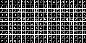
Below is a sample of handwritten digits from the MNIST dataset, which LeNet-5 was designed to classify:
How It Works
1. Normalize the input
The original network receives a 32 × 32 grayscale image. Padding a 28 × 28 digit into this larger field places the character away from the boundary.
2. Extract and downsample features
| Layer | Operation | Output | Kernel / stride |
|---|---|---|---|
| C1 | Convolution | 28 × 28 × 6 | 5 × 5 / 1 |
| S2 | Trainable subsampling | 14 × 14 × 6 | 2 × 2 / 2 |
| C3 | Partially connected convolution | 10 × 10 × 16 | 5 × 5 / 1 |
| S4 | Trainable subsampling | 5 × 5 × 16 | 2 × 2 / 2 |
| C5 | Convolution | 1 × 1 × 120 | 5 × 5 |
| F6 | Fully connected | 84 | — |
| Output | Gaussian/RBF units | 10 | — |
C1 detects simple local patterns. S2 reduces each map's width and height. C3 combines selected S2 maps rather than connecting every input map to every output map, and S4 downsamples again. Because C5 uses 5 × 5 kernels on 5 × 5 inputs, each of its 120 units sees the complete S4 representation.
3. Produce a class score
F6 maps the 120 C5 values to 84 activations. The original output layer compares that representation with learned radial-basis-function prototypes for ten classes. Modern recreations often replace this detail with a conventional linear layer and softmax, so they are LeNet-like rather than exact replicas.
4. Train end to end
Backpropagation adjusts the convolution kernels, trainable subsampling parameters, and classifier together. The original uses scaled hyperbolic-tangent activations rather than ReLU and has roughly 60,000 trainable parameters.
Why It Works
- Local receptive fields: A unit only needs to inspect a small neighborhood to recognize a stroke or edge.
- Weight sharing: One kernel is reused across a feature map, sharply reducing parameters and making feature detection translation-equivariant.
- Hierarchical composition: Later layers combine simple strokes into larger digit parts.
- Downsampling: Subsampling reduces computation and gives some tolerance to small shifts and distortions; it does not make the network perfectly translation-invariant.
- End-to-end learning: The feature extractor is optimized for the recognition task rather than hand-designed separately.
Limitations
- The small capacity and fixed 32 × 32 grayscale input suit relatively simple document images, not modern high-resolution visual tasks.
- Tanh activations can saturate and weaken gradients, making substantially deeper versions difficult to optimize.
- The original design predates batch normalization, dropout, and residual connections.
- Subsampling discards spatial detail, and its shift tolerance is limited.
- Its specialized Gaussian output is uncommon in current classifiers and is often omitted in implementations.
Related
- CNN
- MLP
- Vision Transformer
- Convolution
- Pooling
- AlexNet (2012) scaled the convolutional recipe to ImageNet; VGGNet made it deeper; ResNet added residual paths; MobileNet later emphasized efficiency.
Sources
- Gradient-Based Learning Applied to Document Recognition - Original LeNet-5 paper by LeCun et al.
- LeNet-5 Demo - Official demo page from Yann LeCun
- LeNet - Wikipedia